In January 2025, Kaggle ran a playground series competition to forecast multiple years’ worth of sticker sales in different countries. For each id row, you have to predict the num_sold which represents the number of stickers sold for each product type per store in each country.
This notebook walks through building, deploying and serving a machine learning model for forecasting sticker sales.
I do my tabular data preprocessing and build my model using fastai, I then push my training, test and validation data to modal and run a script which runs the training job on modal cloud.
Now we can proceed to run some python scripts which deploy and serve the same model to a web endpoint in modal as we shall see below. I can then pass new data without a sales column to this API and expect it to return the same data with new sales predictions in a new num_sold column.
Modal is a serveless cloud platform that enables us to run and execute any python code in the cloud without having to manage infrastructure. Modal makes it easy to attach GPU’S with just one line of code and can serve our functions as web endpoints.
Modal makes deploying ML models simple with:
Containerized environments defined in code
Seamless scaling
GPU support (when needed)
Easy endpoint creation
I previously showed how to train, serve and deploy a machine learning model to a live API endpoint with bentoml and bentocloud here.
The solution we are building below will allow us to:
Train a gradient boosting model to predict sticker sales
Use Modal for serverless deployment
Create an API endpoint for predictions
Visualize results with a Streamlit dashboard.
After we are done deploying and serving our machine learning model, we build a UI where we pass in the API link. This can be used to make calls to the API from our streamlit dashboard.
Streamlit is an open source framework that we can use to quickly build web applications.
Once we are done building our web application, we can pass in our data for a single prediction using a form etc.
We can also do batch prediction by passing in a csv file of the new data you want it will make predictions on.
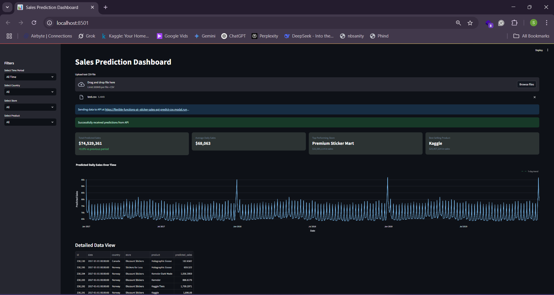
Our batch prediction solution looks like below when we are done.
Sticker sales forecasting dashboard built with streamlit
As you can see above, once we pass in previously unseen data, our model returns new predictions for the number of stickers to be sold.
Evaluation
The competition submissions were evaluated on the Mean Absolute Percentage Error (MAPE) metric which expresses the average absolute error as a percentage of the actual values, making it easy to understand the relative size of errors.
For example, if you predict a value of 90 when the actual is 100, the percentage error is 10%, but if you predict 110 when the actual is 100, the percentage error is also 10%. MAPE averages these absolute percentage errors across all observations.
NB: The data for this competition was synthentically generated but was made to contain real world patterns and effects that you might see in real world data such as seasonality, weekend and holiday effect, etc.
Let’s get started!
Project Structure
We start by creating our project file structure which should follow the structure below. Follow this and create the neccesary directories and files.
The training data, train.csv shall automatically be loaded into the data folder as we shall see in the Extract and Load section below hence we just need to create the data folder.
sticker_sales_model_deployment/
├── data/
    └── train.csv                  # Training and test data
    └── test.csv                   # Test data
    └── sample_submission.csv      # sample submission data for kaggle
    └── transformed_data.csv       # Training data extracted from airbyte data - Approach 2
    └── local_filename.csv         # airbyte data from s3 - ELT job
    └── output.csv                 # Training data extracted from airbyte data - Approach 1
├── data_upload.py                 # Upload data to modal cloud
├── train.py                       # Modal model training
├── serve.py                       # Create API service with Modal
├── test_modal_api.py              # Modal API test
└── ui/
    └── streamlit_ui.py            # Streamlit dashboard
Setting Up Your Environment
Let’s start by setting up our environment. We start by logging into modal by running modal setup via our terminal.
We then install the libraries we need for this project by running the below pip installations via your terminal.
You can do the same installation by running pip install catboost seaborn xgboost lightgbm fastkaggle -Uqq fastbook polars tqdm gradio dash streamlit plotly requests boto3 modal bentoml pandas via your terminal in your home directory which in this case would be sticker_sales_model_deployment/.
Airbyte - An open source data movement infrastructure for building extract and load (EL) data pipelines.
To replicate/mirror how we would build & work with systems in real life, where data sources might be in different data sources such as ERP systems, spreadsheet software, social media apps, websites, etc.
I use Airbyte, an open source tool that can be used to extract and load data from one source to another to build data pipelines.
This shows how one would go about extracting data from different sources to a single data warehouse / lake. With this we can always easily pull our neccesary data into our native training enviroment.
To demonstrate this in our example, we uploaded our training csv data into a google sheet and then pulled it AWS S3. Airbyte is well suited to handle this.
Once the data has been extracted from google sheets to AWS S3, we run the code below to pull the data from AWS S3 into our notebook and native training enviroment.
# Method 1: Download file to local and then reads3_client.download_file('flexible-functions', 'sticker-sales/train.csv/ss_train.csv', 'data/local_filename_ss.csv')airbyte_df = pd.read_csv('data/local_filename_ss.csv')
Our data is in the _airbyte_data column, so lets go ahead and extract it. We have a few ways we can do this.
Approach 1
# Extract the JSON blobs from the '_airbyte_data' columndata = airbyte_df['_airbyte_data'].apply(json.loads)# Convert the extracted JSON data into a DataFrameextracted_df = pd.json_normalize(data)# Save the extracted DataFrame to a CSV file in the data folderextracted_df.to_csv("data/output.csv", index=False)print("Data successfully extracted and saved to data/output.csv")output_df = pd.read_csv('data/output.csv')output_df.head()
Approach 2
We can load our data in a more optimal way. Lets do that below
def transform_airbyte_data(input_file, output_file):""" Transform Airbyte raw data format back to original tabular format Parameters: input_file (str): Path to the input file (CSV or JSON) from Airbyte output_file (str): Path to save the transformed CSV file Returns: pd.DataFrame: The transformed DataFrame """ file_ext = os.path.splitext(input_file)[1].lower()# Read the data based on file typeif file_ext =='.csv': df = pd.read_csv(input_file)elif file_ext =='.json': df = pd.read_json(input_file, lines=True) # Assuming JSONL formatelse:raiseValueError(f"Unsupported file extension: {file_ext}. Use .csv or .json")# Check if the data is in Airbyte format airbyte_columns = [col for col in df.columns if col.startswith('_airbyte_')]if'_airbyte_data'in df.columns:# If *airbyte*data is a string column, parse it to dictionariesif df['_airbyte_data'].dtype =='object'andisinstance(df['_airbyte_data'].iloc[0], str): df['_airbyte_data'] = df['_airbyte_data'].apply(json.loads)# Extract the data from *airbyte*data column extracted_data = pd.json_normalize(df['_airbyte_data'])# Convert numeric columns if neededfor col in extracted_data.columns:if col in ['id', 'num_sold']:try: extracted_data[col] = pd.to_numeric(extracted_data[col])except:pass# Keep as string if conversion fails# Save the result extracted_data.to_csv(output_file, index=False)print(f"Transformed data saved to {output_file}")return extracted_dataelse:print("Data doesn't appear to be in Airbyte format. No transformation needed.") df.to_csv(output_file, index=False)return df
# Example usageif__name__=="__main__":# Use paths in the data folder input_file ="data/local_filename_ss.csv"# or .json output_file ="data/transformed_data.csv" transformed_df = transform_airbyte_data(input_file, output_file) transformed_df.head()
Load data
We only did an ELT job for the training dataset for demonstration
For the test and sample submission file, we shall load them from the local files already available in the data/ folder.
# For a specific column (e.g., column 'A')missing_values_count = train_df['num_sold'].isnull().sum()missing_values_count
train_df['num_sold'].isnull().mean() *100
Data Upload - data_upload.py
We are now going to start by uploading our data to modal using volumes. To quote the modal documentation
Modal Volumes provide a high-performance distributed file system for your modal applications. They are designed for write-once, read-many I/O workloads, like creating machine learning model weights and distributing them for inference.
Uploading our data will enable our training function that we run later to access the data it will need to train our machine learning model.
NB: You can achieve the same data upload functionality using modal Images by using the image.add_local_dir and image.add_local_file image builder methods. This can be done by creating an image that has our data like below
sticker_data_image = (
    modal.Image.debian_slim()
    .pip_install(["pandas", "numpy", "xgboost", "bentoml"])
    # Add your local data directory to the image
    .add_local_dir("./data", remote_path="/data")
)
For this example, I shall be uploading my data using modal volumes as opposed to using images.
Navigate to your data_upload.py file and paste the below code which whose purpose we shall explain in detail.
import modalimport sysfrom pathlib import Path# Create an app for the data upload app = modal.App("sticker-data-upload")
Here we are initializing a modal application named sticker-data-upload.
Modal is a cloud platform that lets you run Python functions in the cloud. The App class is used to define a Modal application which is just a group of functions and classes that are deployed together.
# Create a volume to persist datavolume = modal.Volume.from_name("sticker-data-volume", create_if_missing=True)
We then define our volume with modal.Volume.from_name which creates a persistent storage volume in modal named sticker-data-volume. The create_if_missing=True flag means it will create the volume if it doesn’t already exist.
Volumes in modal are like shared disk space that can persist between function runs.
Modal Data Upload
@app.function(volumes={"/data": volume})def upload_data(local_data_path):import shutilimport os# Ensure the destination directory exists os.makedirs("/data", exist_ok=True)# Copy all files from the local data directory to the volumeforfilein Path(local_data_path).glob("*"): dest =f"/data/{file.name}"iffile.is_file(): shutil.copy(file, dest)print(f"Copied {file} to {dest}")# List files to confirm uploadprint("\nFiles in Modal volume:")forfilein Path("/data").glob("*"):print(f" - {file}")
Remember our modal app can consist of various functions and classes. To explicitly register an object with the app, we use the @app.function() decorator.
We can now define the function, upload_data to upload our data. The function takes in one argument, local_data_path which is the path to the directory on our local machine that contains the files we would like to upload.
Inside the function, start by creating the /data directory if it does not exist. We then iterate through our local file directory.
For each file, we create a destination path in our modal volume, and if it is a file, copy it from our local directory to our previously defined modal volume and then it prints a confirmation message.
Finally, It prints a list of all files in the volume.
@app.local_entrypoint()def main():iflen(sys.argv) >1: data_path = sys.argv[1]else: data_path ="./data"# Default pathprint(f"Uploading data from {data_path}") upload_data.remote(data_path)
The @app.local_entrypoint() decorator defines a Command Line entry point for our modal app and it marks a function, in this case main to be executed locally.
This function then parses command-line arguments such as the data path, print a local message, and then triggers the actual data uploading process.
Our function, main triggers our function upload_data to be executed remotely in the modal cloud by calling upload_data.remote(data_path) .
To upload the data, run python data_upload.py ./data via the terminal to trigger the data upload.
Model Training - train.py
Next, we’ll create a script to train our forecasting model. Navigate to your train.py file and paste the code in the below model training section whose code i shall explain.
#import modal#import pandas as pd#import numpy as np#from fastai.tabular.all import * # Move this import to the top level#import xgboost as xgb#import bentoml#from pathlib import Path#import os#import pickle# Define Modal resourcesapp = modal.App("sticker-sales-forecast")
Above, we define a modal app called sticker-sales-forecast.
We then define an image which is a snapshot of our container’s filesystem state.
We can easily add any third-party packages like torch, pandas by passing in all the packages we need to the pip_install method of an image as shown above.
After defining our dependencies, we call and attach an existing volume called sticker-data-volume which we previously defined when doing our data upload.
This contains the data needed for our model training in the train_model function defined below.
We define our @app.function decorator passing in our specified image and volume mounted at “/data”.
Forecasting Model Training Function
# Define paths for pickle-based model savingMODEL_PATH ="/data/sticker_sales_model.pkl"PREPROC_PATH ="/data/sticker_sales_preproc.pkl"@app.function(image=image, volumes={"/data": volume})def train_model():# No need to import fastai.tabular.all here since we moved it to the top# Set up paths path = Path('/data/')# Check if data files existprint("Files available in volume:")forfilein path.glob("*"):print(f" - {file}")# Load dataprint("Loading data...") train_df = pd.read_csv(path/'train.csv', index_col='id') test_df = pd.read_csv(path/'test.csv', index_col='id')# Data preprocessingprint("Preprocessing data...") train_df = train_df.dropna(subset=['num_sold']) train_df = add_datepart(train_df, 'date', drop=False) test_df = add_datepart(test_df, 'date', drop=False)# Feature preparation cont_names, cat_names = cont_cat_split(train_df, dep_var='num_sold') splits = RandomSplitter(valid_pct=0.2)(range_of(train_df)) to = TabularPandas(train_df, procs=[Categorify, FillMissing, Normalize], cat_names=cat_names, cont_names=cont_names, y_names='num_sold', y_block=CategoryBlock(), splits=splits) dls = to.dataloaders(bs=64)# Prepare training data X_train, y_train = to.train.xs, to.train.ys.values.ravel() X_test, y_test = to.valid.xs, to.valid.ys.values.ravel()# Train XGBoost modelprint("Training XGBoost model...") xgb_model = xgb.XGBRegressor() xgb_model = xgb_model.fit(X_train, y_train)# Save model with BentoMLprint("Saving model with BentoML...") model_tag = bentoml.xgboost.save_model("sticker_sales_v1", xgb_model, custom_objects={"preprocessor": {"cont_names": cont_names,"cat_names": cat_names } } )# Save model with pickleprint(f"Saving model with pickle to {MODEL_PATH}...")withopen(MODEL_PATH, 'wb') as f: pickle.dump(xgb_model, f)# Save preprocessing info separatelyprint(f"Saving preprocessing info to {PREPROC_PATH}...") preproc_info = {"cont_names": cont_names,"cat_names": cat_names,"procs": [Categorify, FillMissing, Normalize] }withopen(PREPROC_PATH, 'wb') as f: pickle.dump(preproc_info, f)# Ensure changes are committed to the volume volume.commit()print(f"Model saved: {model_tag} and to pickle files")returnstr(model_tag)
In our code above, I am defining a function train_model.
In this function, I start by setting up the paths and loading the training and test data into their respective data frames, train_df and test_df.
I then do some basic preprocessing steps on our data frames.
First, from our exploratory data analysis above, I noticed that our target column, num_sold has missing values which would intefere with our model training, so first we handle this.
We can deal with these missing values with several techniques like filling in with the mean, median, or a random value. From testing, I noticed the best strategy for this is to drop all the rows with missing values by running train_df = train_df.dropna(subset=['num_sold']).
We then use the add_datepart helper function from fast.ai to add columns/features relevant to the date column in a data frame if available. This is defined using add_datepart (df, field_name, prefix=None, drop=True, time=False).
For example, if we have a date column with a row that has 2019-12-04. We can derive new columns from that date such as Year, Month, Day, Dayofweek, Is_month_start, Is_quarter_end, etc.
Our machine learning model expects our training data to be in a certain format. Luckily, fastai has functions which we shall see below that can help transform this raw data into a format that can be efficiently and effectively processed by a neural network.
We then go on to define categorical and continuous variables, I use the fastai cont_cat_split function to separate my dataset variables into categorical and continuous variables based of the cardinality of my column values.
cont_cat_split takes an argument max card whose default is 20. If the number of unique values exceeds 20 (max_card value) for a particular column, that column is considered continuous, and vice versa.
I then use RandomSplitter, a fastai function that splits our training data into new training and validation sets.
It separates the training dataset into training and validation sets based on the value of the argument valid_pct.
We can now use fastai’s TabularPandas class to create a TabularPandas object that applies given preprocessing steps to our data.
This creates a data frame wrapper that takes in different arguments and knows which columns are categorical and continuous. I also define the target variable, y_name, the type of target, the problem we are dealing with such as a regression problem in this case, and the way to split our data which was previously defined in the splits above.
I define a list of preprocessing steps, Procs, to be taken on our data which we pass to our TabularPandas object. Procs contains the below preprocessing steps.
Categorify deals with the categorical variables and converts each category into a list of indexable numerical integers, creating numerical input which is required by our model. Each category corresponds to a different number.
FillMissing as its name suggests, fills in the missing values in columns with continuous values. This can be filled in with the median, mode of that column, or a constant, with the default being the median value for that particular column.
FillMissing supports using the mode and a constant as strategies for dealing with missing values. We can do this by changing the FillMissing argument fill_strategy to mode or constant.
Normalize puts the continuous variables between a standardized scale without losing important information by subtracting the mean and dividing by the standard deviation.
We can now define a DataLoader which is an extension of PyTorch’s DataLoaders class albeit with more functionality. This takes in our data above from the TabularPandas object and prepares it as input for our model passing it in batches which we defined by our batch size set by the bs argument.
The DataLoaders and TabularPandas objects allow us to build data objects we can use for training without specifically changing the raw input data.
The dataloader then acts as input for our models.
To use other libraries with fastai, I extract the x’s and y’s from my TabularPandas object which I used to preprocess the data. I can now directly use the training and validation set values I extracted above as direct input for decision trees and gradient-boosting models.
An instance of XGBRegressor is then created with default parameters, and a model is trained by calling .fit() with the training features (X_train) and target values (y_train). The model is finally serialized and saved to the bentoML model store.
Entry Point
@app.local_entrypoint()def main():# Train the model remotelyprint("Starting model training on Modal...") model_tag = train_model.remote()print(f"Model training completed. Model tag: {model_tag}")print(f"Model and preprocessing info also saved as pickle files at {MODEL_PATH} and {PREPROC_PATH}")
Above, we define our entry point.
As explained before the @app.local_entrypoint() decorator, declared above makes this function the entry point when you run the script locally and it triggers the remote execution of the train_model function in modal cloud by calling train_model.remote() within our main function.
@app.local_entrypoint()
def main():
    # Train the model remotely
    print("Starting model training on Modal...")
    model_tag = train_model.remote()
    print(f"Model training completed. Model tag: {model_tag}")
Now run python train.py via the terminal to trigger the machine learning model training and saving in modal cloud.
Trained model serving and deployment - serve.py
After training our model, we can proceed to deploy and serve our trained machine learning model.
To do this, go to the serve.py file and paste all the code in the below model serving and deployment section.
Just like before, we create a modal app called sticker-sales-api which acts as the container for all the functions that will be deployed.
#import modal#import pandas as pd#import numpy as np#from fastapi import File, UploadFile, Form, HTTPException#import io# Create app definitionapp = modal.App("sticker-sales-api")# Define base image with all dependenciesbase_image = (modal.Image.debian_slim() .pip_install("pydantic==1.10.8") .pip_install("fastapi==0.95.2") .pip_install("uvicorn==0.22.0") .pip_install("bentoml==1.3.2") .pip_install([ "xgboost==1.7.6","scikit-learn==1.3.1","pandas","numpy", ]))# Create the fastai image by extending the base imagefastai_image = (base_image .pip_install(["fastai", "torch"]))
We then go ahead and define two separate container images.
The main image, base_image includes dependencies for the API (FastAPI, pydantic, uvicorn) plus modal-related packages (BentoML, XGBoost, scikit-learn).
A separate fastai_image is created to avoid dependency conflicts, as fastai has specific requirements for torch and other packages.
# Create volume to access datadata_volume = modal.Volume.from_name("sticker-data-volume")
Just like before, we call and attach an exisiting volume called sticker-data-volume.
# Simple health endpoint@app.function(image=base_image)@modal.fastapi_endpoint(method="GET")def health():"""Health check endpoint to verify the API is running"""return {"status": "healthy", "service": "sticker-sales-api"}
We define a health endpoint to provide a simple way to check if our API service is alive and functioning correctly. We can use this to verify our service is available without needing to test the full prediction functionality.
Forecasting Model Serving Function
# Function to train and save model @app.function(image=fastai_image, volumes={"/data": data_volume})def serve_model():"""Load or train an XGBoost model"""import xgboost as xgbfrom fastai.tabular.allimport add_datepart, TabularPandas, cont_cat_splitfrom fastai.tabular.allimport Categorify, FillMissing, Normalize, CategoryBlock, RandomSplitter, range_offrom pathlib import Pathimport pickleimport osimport bentoml# Model tag used in train.py model_tag ="sticker_sales_v1"# Create a path to save the model for future use model_path ="/data/sticker_sales_model.pkl"try:# First attempt: Try loading from BentoMLprint(f"Attempting to load model from BentoML with tag '{model_tag}'...")try: bento_model = bentoml.xgboost.load_model(model_tag)print(f"Successfully loaded model from BentoML.")return bento_modelexceptExceptionas e:print(f"Could not load from BentoML: {str(e)}")# Second attempt: Try loading from pickleif os.path.exists(model_path):print(f"Loading existing model from pickle at {model_path}")withopen(model_path, 'rb') as f: model = pickle.load(f)return model# Third attempt: Train a new model if neither option workedprint("No existing model found. Training new model...")# Load and preprocess training data path = Path('/data/')print("Loading training data...") train_df = pd.read_csv(path/'train.csv', index_col='id')# Drop rows with missing target values train_df = train_df.dropna(subset=['num_sold'])# Add date featuresprint("Preprocessing data...") train_df = add_datepart(train_df, 'date', drop=False)# Feature preparation cont_names, cat_names = cont_cat_split(train_df, dep_var='num_sold') splits = RandomSplitter(valid_pct=0.2)(range_of(train_df))# Create TabularPandas processor to = TabularPandas(train_df, procs=[Categorify, FillMissing, Normalize], cat_names=cat_names, cont_names=cont_names, y_names='num_sold', y_block=CategoryBlock(), splits=splits)# Prepare training data X_train, y_train = to.train.xs, to.train.ys.values.ravel()# Train a simple XGBoost modelprint("Training XGBoost model...") xgb_model = xgb.XGBRegressor(n_estimators=100) xgb_model.fit(X_train, y_train)# Save model to both formats# 1. Save to BentoMLprint(f"Saving model to BentoML with tag '{model_tag}'...") bentoml.xgboost.save_model( model_tag, xgb_model, custom_objects={"preprocessor": {"cont_names": cont_names,"cat_names": cat_names } } )# 2. Save to pickleprint(f"Saving model to pickle at {model_path}")withopen(model_path, 'wb') as f: pickle.dump(xgb_model, f)# Save preprocessing info separately preproc_path ="/data/sticker_sales_preproc.pkl"print(f"Saving preprocessing info to {preproc_path}...") preproc_info = {"cont_names": cont_names,"cat_names": cat_names,"procs": [Categorify, FillMissing, Normalize] }withopen(preproc_path, 'wb') as f: pickle.dump(preproc_info, f)# Ensure changes are committed to the volume volume.commit()print("Model training and saving complete!")return xgb_modelexceptExceptionas e:import tracebackprint(f"Error loading/training model: {str(e)}")print(traceback.format_exc())raise
Above we define a function serve_model
First, it checks if a trained model exists in our current model_path in our modal volume.
If found, it loads the existing model; if not, it trains a new one. This is a fallback mechanism built into the serving API that first checks if a model exists at a specific path on the volume.
This ensures the API endpoint can always return predictions, even if the scheduled training hasn’t run yet.
# CSV upload endpoint @app.function(image=fastai_image, volumes={"/data": data_volume})@modal.fastapi_endpoint(method="POST")asyncdef predict_csv(file: UploadFile = File(...)):"""API endpoint for batch predictions from a CSV file"""import xgboost as xgbimport ioimport picklefrom fastai.tabular.allimport add_datepart, TabularPandas, cont_cat_splitfrom fastai.tabular.allimport Categorify, FillMissing, Normalize, CategoryBlock, RandomSplitter, range_offrom pathlib import Pathtry:# First, train or load model model = serve_model.remote()# Read uploaded CSV file content contents =awaitfile.read()# Parse CSV datatry: test_df = pd.read_csv(io.BytesIO(contents))exceptExceptionas e:return {"success": False,"error": f"Failed to parse uploaded CSV: {str(e)}" }# Load the training data for preprocessing path = Path('/data/') train_df = pd.read_csv(path/'train.csv', index_col='id') train_df = train_df.dropna(subset=['num_sold'])# Add date features to both datasets train_df = add_datepart(train_df, 'date', drop=False) test_df = add_datepart(test_df, 'date', drop=False)# Feature preparation cont_names, cat_names = cont_cat_split(train_df, dep_var='num_sold') splits = RandomSplitter(valid_pct=0.2)(range_of(train_df))# Create TabularPandas processor to = TabularPandas(train_df, procs=[Categorify, FillMissing, Normalize], cat_names=cat_names, cont_names=cont_names, y_names='num_sold', y_block=CategoryBlock(), splits=splits)# Create a test dataloader dls = to.dataloaders(bs=64) test_dl = dls.test_dl(test_df)# Make predictions using our model predictions = model.predict(test_dl.xs)# Return the predictions as a simple listreturn predictions.tolist()exceptExceptionas e:import tracebackreturn {"success": False,"error": f"Error processing CSV: {str(e)}","traceback": traceback.format_exc() }
We then define a predict_csv function which creates a REST API endpoint that enables batch predictions for multiple sticker sales records via a CSV file upload.
predict_csv starts by calling the serve_model function previously defined to be executed. This loads up our machine learning model if we have one available or trains a new one as we saw before.
We then read in the uploaded file csv file as bytes, wrap it in an in-memory buffer using BytesIO, and safely parse it into a pandas DataFrame with error handling.
Above, we load our training data to enable us to recreate the preprocessing steps using TabularPandas. This is necessary because Fastai needs the original transformations to correctly preprocess the new test data and requires this to generate the test_dl from the incoming test data
When making predictions with tabular machine learning models, we must apply the exact same preprocessing transformations to new data that were used during training.
With this we can now add date-related features with add_datepart, apply the same preprocessing transformations ( Categorify, FillMissing,Normalize) that were used during training and finally create a test dataloader, test_dl with the proper format expected by the model.
We can now make predictions by running the model on the prepared data which returns the sales predictions as a JSON array that can be consumed by clients.
The above ensures consistent processing between training and inference, but creates unnecessary overhead and is probably not the most optimal way of handling the preprocessing as it requires us to reload and reprocess the training data for each prediction.
So we can try out another implementation and try to leverage our previously saved preprocessing information at inference time as opposed to loading the training dataset everytime.
We previously saved our steps in the serve_model function where we did this
To do this, we shall redefine predict_csv to add the use of the saved preprocessing steps with the previous implementation as a backup if the preprocessing information is not available.
# CSV upload endpoint - with debugging info (commented out)@app.function(image=fastai_image, volumes={"/data": data_volume})@modal.fastapi_endpoint(method="POST")asyncdef predict_csv(file: UploadFile = File(...)):"""API endpoint for batch predictions from a CSV file using cached preprocessing"""import xgboost as xgbimport ioimport pickleimport osimport tracebackfrom fastai.tabular.allimport add_datepart, TabularPandas, cont_cat_splitfrom fastai.tabular.allimport Categorify, FillMissing, Normalize, CategoryBlock, RandomSplitter, range_offrom pathlib import Path# Uncomment for debugging# response_data = {"success": False, "debug_info": {}}try:# Debug information# response_data["debug_info"]["step"] = "Starting prediction process"# First, load or train model model = serve_model.remote()# response_data["debug_info"]["model_loaded"] = True# Read uploaded CSV file content contents =awaitfile.read()# Parse CSV datatry: test_df = pd.read_csv(io.BytesIO(contents))# response_data["debug_info"]["test_columns"] = test_df.columns.tolist()# response_data["debug_info"]["test_shape_before"] = test_df.shapeexceptExceptionas e:return {"success": False,"error": f"Failed to parse uploaded CSV: {str(e)}" }# Add date features to the test dataset test_df = add_datepart(test_df, 'date', drop=False)# response_data["debug_info"]["test_shape_after_datepart"] = test_df.shape# response_data["debug_info"]["test_columns_after_datepart"] = test_df.columns.tolist()# Load the full training data to ensure proper preprocessing path = Path('/data/') train_df = pd.read_csv(path/'train.csv', index_col='id') train_df = train_df.dropna(subset=['num_sold'])# response_data["debug_info"]["train_columns"] = train_df.columns.tolist()# response_data["debug_info"]["train_shape"] = train_df.shape# Add date features to training data train_df = add_datepart(train_df, 'date', drop=False)# response_data["debug_info"]["train_columns_after_datepart"] = train_df.columns.tolist()# Feature preparation cont_names, cat_names = cont_cat_split(train_df, dep_var='num_sold')# response_data["debug_info"]["categorical_features"] = cat_names# response_data["debug_info"]["continuous_features"] = cont_names# Check if test data has all required columns missing_cols = []for col in cat_names + cont_names:if col notin test_df.columns: missing_cols.append(col)if missing_cols:# response_data["debug_info"]["missing_columns"] = missing_cols# Add missing columns with default valuesfor col in missing_cols:if col in cat_names: test_df[col] ="unknown"# Default value for categoricalelse: test_df[col] =0.0# Default value for continuous# response_data["debug_info"]["columns_added"] = missing_cols# Create TabularPandas processor splits = RandomSplitter(valid_pct=0.2)(range_of(train_df)) to = TabularPandas(train_df, procs=[Categorify, FillMissing, Normalize], cat_names=cat_names, cont_names=cont_names, y_names='num_sold', y_block=CategoryBlock(), splits=splits)# Create dataloaders dls = to.dataloaders(bs=64)# Process the test data and make predictions test_dl = dls.test_dl(test_df)# response_data["debug_info"]["test_xs_shape"] = test_dl.xs.shape# Make predictions predictions = model.predict(test_dl.xs)# Return predictions in the format expected by test_modal_api.pyreturn predictions.tolist()# To return structured response with debug info, use this instead:# response_data["success"] = True# response_data["predictions"] = predictions.tolist()# return response_dataexceptExceptionas e:import tracebackreturn {"success": False,"error": f"Error processing CSV: {str(e)}","traceback": traceback.format_exc() }
@app.local_entrypoint()def main():"""Local entrypoint for testing the API"""print("Starting sticker-sales-api...")# Pre-train the model to ensure it existsprint("Training model...") serve_model.remote()print("Model training complete!")print("\nAPI is ready for use at:")print("- Health check: https://flexible-functions-ai--sticker-sales-api-health.modal.run")print("- CSV predictions: https://flexible-functions-ai--sticker-sales-api-predict-csv.modal.run")
The @app.local_entrypoint() carries out a similar function as before where it triggers the remote execution of the serve_model function in modal cloud when we run modal deploy serve.py.
We also print the endpoint information such as the URLs where the deployed API endpoints can be accessed, making it easier for developers to know where to send requests.
This pattern creates a smoother deployment experience where your model is prepared and ready before any user makes their first API call. It’s particularly helpful during initial deployment and testing phases when you want immediate feedback on whether your endpoints are working correctly.
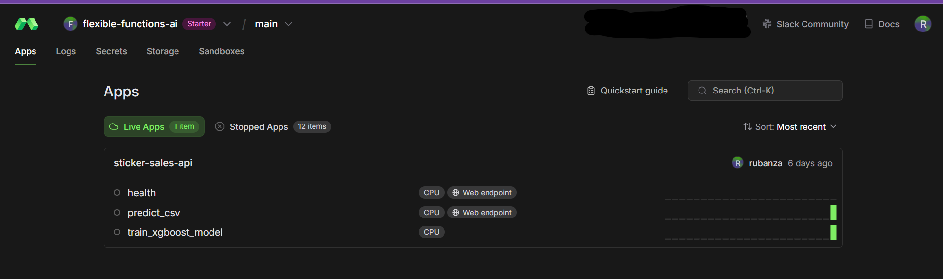
After, we are done running, deploying and serving our app on modal cloud. We can see the App and its API’s in the modal dashboard.
Live sticker sales forecasting app in the Modal dashboard
Above, we essentially create a convenient batch prediction service, allowing our Streamlit dashboard (or any client) to upload a CSV file and immediately get back predictions without having to handle the preprocessing or model loading logic themselves.
We then build a dashboard below with streamlit that uses these predictions to create visualizations, calculate KPIs, and enable interactive filtering of the results but first we shall test our API with a simple script.
Testing the API - test_modal_app.py
Navigate to the home directory and paste the below code in this section into test_modal_api.py. We shall use this to test that our API is working as expected.
The below code makes a request to an API that predicts sticker sales.
import requestsimport pandas as pdimport io# The URL of your CSV prediction endpointurl ="https://flexible-functions-ai--sticker-sales-api-predict-csv.modal.run"# Create a sample CSV with test datatest_data = pd.DataFrame([ {"date": "2023-01-15","country": "US","store": "Store_001","product": "Sticker_A" }, {"date": "2023-01-15","country": "Canada","store": "Discount Stickers","product": "Holographic Goose" }, {"date": "2023-01-16","country": "UK","store": "Sticker World","product": "Kaggle" }])# Save the test data to a CSV file in memorycsv_buffer = io.StringIO()test_data.to_csv(csv_buffer, index=False)csv_bytes = csv_buffer.getvalue().encode()# Prepare the file for uploadfiles = {'file': ('test_data.csv', csv_bytes, 'text/csv')}# Make the prediction requestprint(f"Sending request to {url}...")response = requests.post(url, files=files)# Print the resultprint("Status code:", response.status_code)# Try to parse the JSON responsetry: prediction = response.json()print("Prediction:", prediction)# If the prediction is a list as expectedifisinstance(prediction, list):# Create a DataFrame with predictions result_df = test_data.copy() result_df['predicted_sales'] = predictionprint("\nPrediction results:")print(result_df)exceptExceptionas e:print("Error parsing response:", e)print("Response text:", response.text[:500])
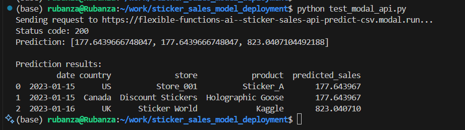
To run the api test, run python test_modal_api.py via the terminal.
This returns predictions, something like below.
Result after running python test_modal_api.py
User Interface with Streamlit - streamlit_ui.py
Finally, let’s create a dashboard with streamlit to visualize our predictions. Streamlit as described before,
is an open-source Python framework for data scientists and AI/ML engineers to deliver dynamic data apps with only a few lines of code.
We navigate to our home directory and navigate to our streamlit code folder named ui. We then paste the code in this section into a file named streamlit_ui.py.
This code enables us to create an interactive dashboard using streamlit that allows users to upload sales data, get predictions from a remote API, and visualize the results.
# Import required librariesimport streamlit as stimport pandas as pdimport requestsimport jsonimport plotly.express as pxfrom datetime import datetimeimport iodef load_and_predict_data(csv_path):""" Sends the test CSV to the API endpoint and gets predictions """try:# Read the CSV file test_df = pd.read_csv(csv_path)# Set the API URL api_url ="https://flexible-functions-ai--sticker-sales-api-predict-csv.modal.run"# Prepare the file for upload using proper multipart/form-data formatwithopen(csv_path, 'rb') as f: files = {'file': ('test_data.csv', f, 'text/csv')}# Make the request st.info(f"Sending data to API at {api_url}...") response = requests.post(api_url, files=files)# Check if the request was successfulif response.status_code ==200:try: result = response.json()# Check if the result is an error messageifisinstance(result, dict) andnot result.get('success', True): st.error(f"Error from API: {result.get('error', 'Unknown error')}") st.error("Using dummy predictions for demonstration") test_df['predicted_sales'] =100# Dummy predictionselse:# Assume the result is a list of predictionsifisinstance(result, list) andlen(result) ==len(test_df): st.success("Successfully received predictions from API") test_df['predicted_sales'] = resultelse: st.warning(f"Unexpected response format. Using dummy predictions.") st.json(result) # Show the actual response test_df['predicted_sales'] =100# Dummy predictionsexceptExceptionas e: st.error(f"Error parsing API response: {str(e)}") st.text(f"Response text: {response.text[:500]}") # Show first 500 chars test_df['predicted_sales'] =100# Dummy predictionselse: st.error(f"API returned status code: {response.status_code}") st.text(f"Response text: {response.text[:500]}") # Show first 500 chars test_df['predicted_sales'] =100# Dummy predictions# Convert date column to datetime test_df['date'] = pd.to_datetime(test_df['date'])return test_dfexceptExceptionas e: st.error(f"Error processing prediction request: {str(e)}")# Return a dummy dataframe for demonstration test_df = pd.read_csv(csv_path) test_df['predicted_sales'] =100# Dummy prediction values test_df['date'] = pd.to_datetime(test_df['date'])return test_df
Above,we define our load_and_predict_data(csv_path) function, which powers the sales forecasting feature in the Streamlit app.
The function reads a test CSV, sends it to an external API for prediction, handles the response, and returns a DataFrame with predicted sales all while implementing proper error handling.
In our function, load_and_predict_data, we
Read the Input CSV
Reads the uploaded CSV file into a pandas DataFrame.
load_and_predict_datafunction enables seamless interaction between the Streamlit app and a backend machine learning model. It is: - Robust: Handles network and response errors gracefully. - User-friendly: Uses Streamlit to notify users of progress or issues. - Fail-safe: Provides dummy predictions if the API fails or returns unexpected results.
def create_dashboard():""" Creates the Streamlit dashboard with enhanced filters, KPI cards, and visualizations """ st.title("Sales Prediction Dashboard")# Add custom CSS for dark theme cards st.markdown(""" <style> .metric-card { background-color: #2C3333; padding: 20px; border-radius: 10px; margin: 10px 0; } .metric-label { color: #718096; font-size: 0.875rem; } .metric-value { color: white; font-size: 1.5rem; font-weight: bold; } .trend-positive { color: #48BB78; } .trend-negative { color: #F56565; } </style> """, unsafe_allow_html=True)# File uploader for the test CSV uploaded_file = st.file_uploader("Upload test CSV file", type=['csv'])if uploaded_file isnotNone:# Save the uploaded file temporarilywithopen('temp_test.csv', 'wb') as f: f.write(uploaded_file.getvalue())# Load data and get predictions df = load_and_predict_data('temp_test.csv')# Convert date column to datetime if not already df['date'] = pd.to_datetime(df['date'])# Creating filters in a sidebar st.sidebar.header("Filters")# Time period filter time_periods = {'All Time': None,'Last Month': 30,'Last 3 Months': 90,'Last Year': 365 } selected_period = st.sidebar.selectbox('Select Time Period', list(time_periods.keys()))# Country filter countries = ['All'] +sorted(df['country'].unique().tolist()) selected_country = st.sidebar.selectbox('Select Country', countries)# Store filter stores = ['All'] +sorted(df['store'].unique().tolist()) selected_store = st.sidebar.selectbox('Select Store', stores)# Product filter products = ['All'] +sorted(df['product'].unique().tolist()) selected_product = st.sidebar.selectbox('Select Product', products)# Apply filters filtered_df = df.copy()# Apply time filterif time_periods[selected_period]: max_date = filtered_df['date'].max() cutoff_date = max_date - pd.Timedelta(days=time_periods[selected_period]) filtered_df = filtered_df[filtered_df['date'] >= cutoff_date]if selected_country !='All': filtered_df = filtered_df[filtered_df['country'] == selected_country]if selected_store !='All': filtered_df = filtered_df[filtered_df['store'] == selected_store]if selected_product !='All': filtered_df = filtered_df[filtered_df['product'] == selected_product]# Calculate metrics for KPI cards total_sales = filtered_df['predicted_sales'].sum() avg_daily_sales = filtered_df.groupby('date')['predicted_sales'].sum().mean()# Calculate period-over-period changesif time_periods[selected_period]: previous_period = filtered_df['date'].min() - pd.Timedelta(days=time_periods[selected_period]) previous_df = df[df['date'] >= previous_period] previous_df = previous_df[previous_df['date'] < filtered_df['date'].min()] prev_total_sales = previous_df['predicted_sales'].sum() sales_change = ((total_sales - prev_total_sales) / prev_total_sales *100if prev_total_sales !=0else0)else: sales_change =0# Create KPI cards using columns col1, col2, col3, col4 = st.columns(4)with col1: st.markdown(f""" <div class="metric-card"> <div class="metric-label">Total Predicted Sales</div> <div class="metric-value">${total_sales:,.0f}</div> <div class="{'trend-positive'if sales_change >=0else'trend-negative'}">{sales_change:+.1f}% vs previous period </div> </div> """, unsafe_allow_html=True)with col2: st.markdown(f""" <div class="metric-card"> <div class="metric-label">Average Daily Sales</div> <div class="metric-value">${avg_daily_sales:,.0f}</div> </div> """, unsafe_allow_html=True)with col3: top_store = (filtered_df.groupby('store')['predicted_sales'] .sum().sort_values(ascending=False).index[0]) store_sales = (filtered_df.groupby('store')['predicted_sales'] .sum().sort_values(ascending=False).iloc[0]) st.markdown(f""" <div class="metric-card"> <div class="metric-label">Top Performing Store</div> <div class="metric-value">{top_store}</div> <div class="metric-label">${store_sales:,.0f} in sales</div> </div> """, unsafe_allow_html=True)with col4: top_product = (filtered_df.groupby('product')['predicted_sales'] .sum().sort_values(ascending=False).index[0]) product_sales = (filtered_df.groupby('product')['predicted_sales'] .sum().sort_values(ascending=False).iloc[0]) st.markdown(f""" <div class="metric-card"> <div class="metric-label">Best Selling Product</div> <div class="metric-value">{top_product}</div> <div class="metric-label">${product_sales:,.0f} in sales</div> </div> """, unsafe_allow_html=True)# Group by date and calculate daily total predicted sales daily_sales = filtered_df.groupby('date')['predicted_sales'].sum().reset_index()# Create the line chart using Plotly with dark theme fig = px.line( daily_sales, x='date', y='predicted_sales', title='Predicted Daily Sales Over Time' )# Update layout for dark theme fig.update_layout( template="plotly_dark", plot_bgcolor='rgba(0,0,0,0)', paper_bgcolor='rgba(0,0,0,0)', xaxis_title="Date", yaxis_title="Predicted Sales", hovermode='x unified', showlegend=True, legend=dict( orientation="h", yanchor="bottom", y=1.02, xanchor="right", x=1 ) )# Add trend line fig.add_scatter( x=daily_sales['date'], y=daily_sales['predicted_sales'].rolling(7).mean(), name='7-day trend', line=dict(dash='dash', color='#48BB78'), visible='legendonly' )# Display the plot st.plotly_chart(fig, use_container_width=True)# Display detailed data view st.subheader("Detailed Data View") st.dataframe( filtered_df.sort_values('date'), hide_index=True )if__name__=="__main__":# Set page configuration at the very beginning st.set_page_config( page_title="Sales Prediction Dashboard", page_icon="📊", layout="wide", initial_sidebar_state="expanded" ) create_dashboard()
Above, we define another function named create_dashboard() where we build a rich, interactive sales prediction dashboard using Streamlit with support for uploading data, filtering, KPI cards, and time series visualizations.
Sets the Streamlit app layout and starts the dashboard when the script is run directly.
The create_dashboard() function integrates: - Data upload and real-time API predictions - User-driven filtering of predictions - Insightful KPIs with stylish dark-themed cards - Interactive time series plots and a raw data table
It’s a modular and user-friendly interface that enables stakeholders to explore predictive insights across time, location, and product dimensions.
Now you can navigate to the terminal, and run streamlit run streamlit_ui.py to run the streamlit app.
It brings up an option to upload a csv file. We upload our test set csv file should looks like the test_df below.
test_df.head()
date
country
store
product
id
230130
2017-01-01
Canada
Discount Stickers
Holographic Goose
230131
2017-01-01
Canada
Discount Stickers
Kaggle
230132
2017-01-01
Canada
Discount Stickers
Kaggle Tiers
230133
2017-01-01
Canada
Discount Stickers
Kerneler
230134
2017-01-01
Canada
Discount Stickers
Kerneler Dark Mode
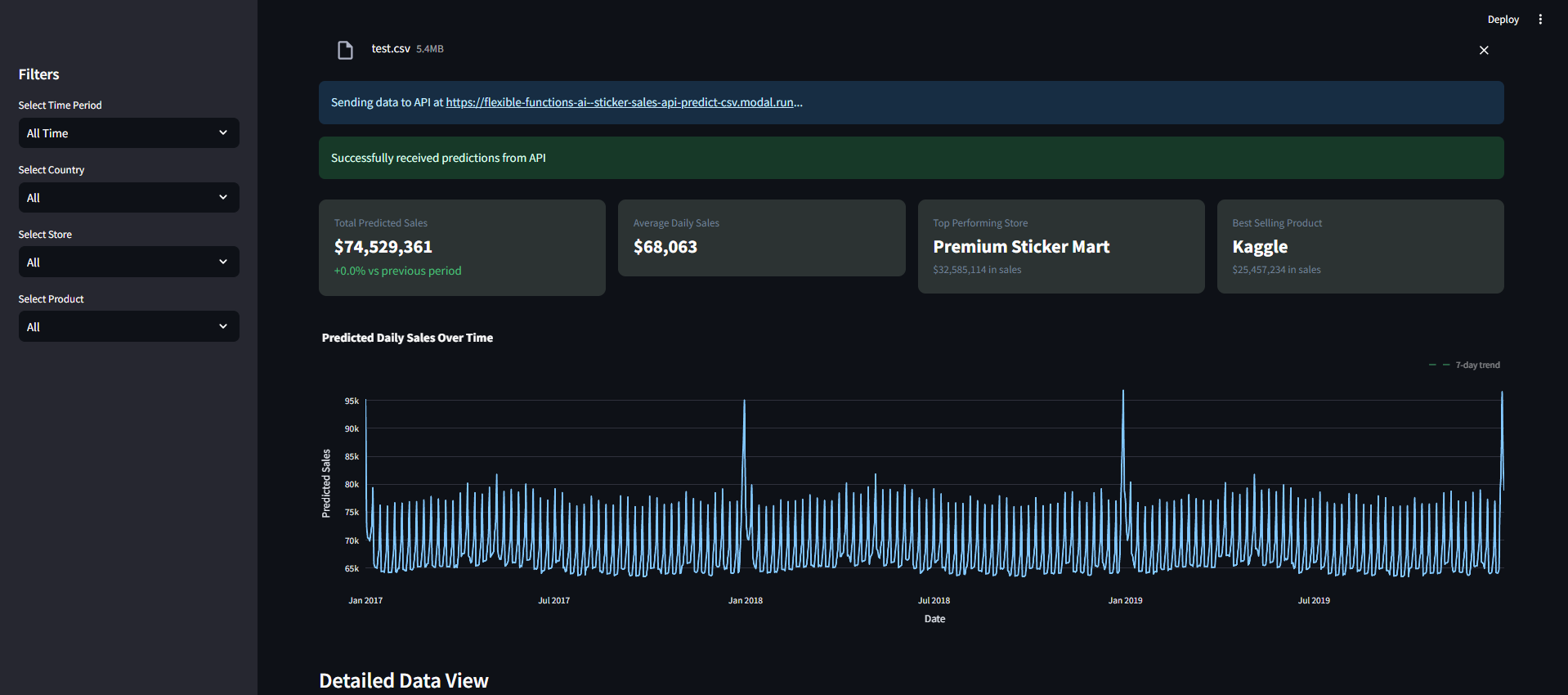
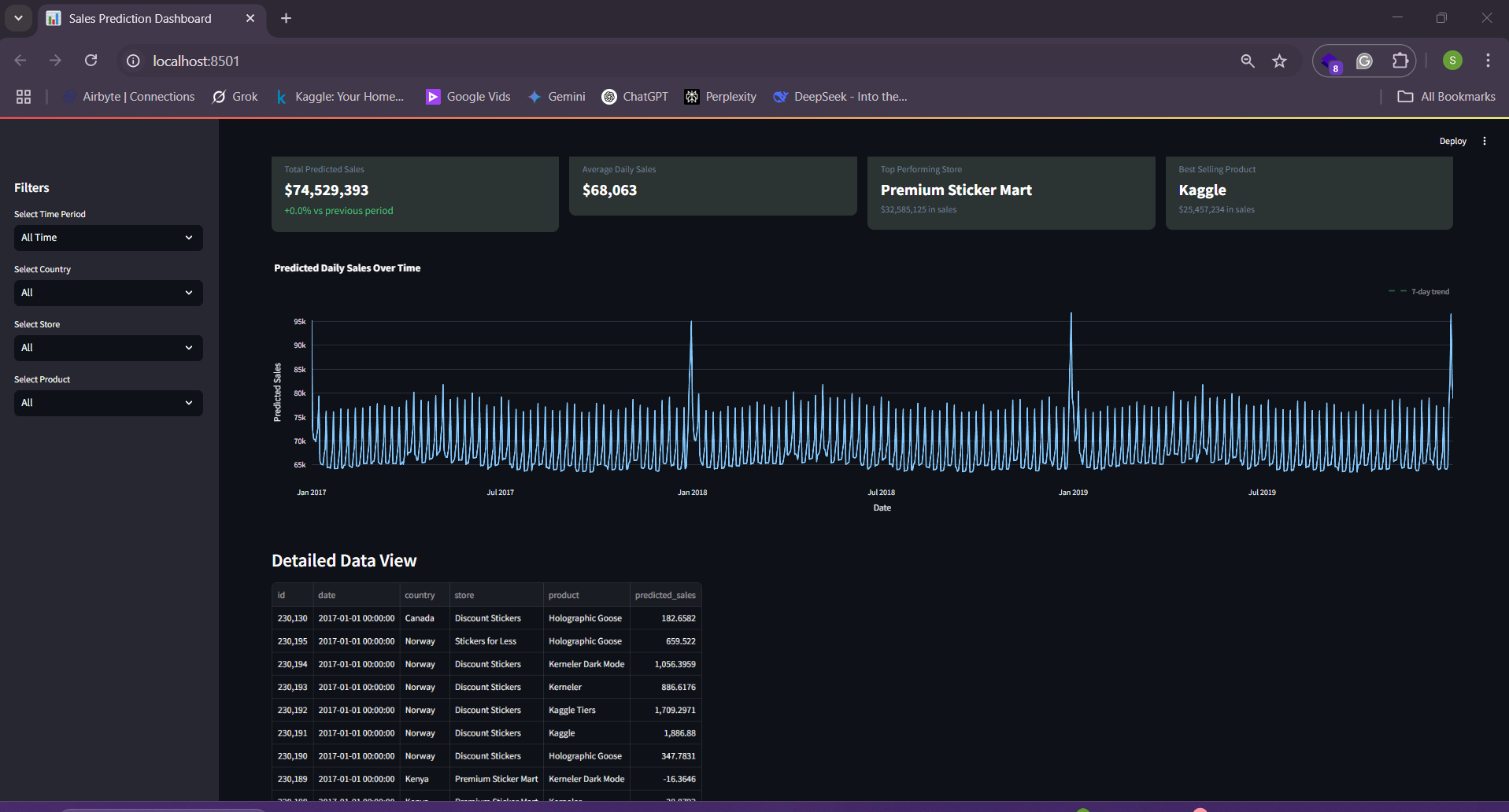
Once we upload our file, the data is sent to the batch prediction api and it returns predictions for the number of sticker sold per day for each product type in each country and for each shop as we can see below.
Sticker sales forecasting dashboard built with streamlit KPI Cards and plot
Sticker sales forecasting dashboard built with streamlit with detailed data view
Running the Entire Pipeline
Here’s how to run the entire pipeline:
Upload data to Modal:
python data_upload.py data/
Train the model on Modal:
python train.py
Deploy the API on Modal:
python serve.py
Run the Streamlit dashboard:
cd uistreamlit run streamlit_ui.py
Key Benefits of This Approach
Serverless Training and Deployment: Modal handles all infrastructure, scaling, and container management.
Production-Ready API: The API is automatically served with proper endpoints, error handling, and authentication.
Separation of Concerns: Data preprocessing, model training, and serving are cleanly separated.
Interactive Dashboard: Stakeholders can visualize predictions without technical knowledge.
Reproducibility: The entire pipeline is defined in code, making it easy to reproduce.
Improvements
Adding a feature store - I shall be adding a feature store in v2 of this blog. This will help with consistent feature engineering and avoid duplicating the same processing logic in different scripts, etc.
Improving the underlying model - I used a basic XGBoost model for this for purposes of ease and speed. I expect to update this to use an ensemble of gradient boosting machines (XGBoost, CatBoost and LightGBM), stacking, etc so as to get improved model predictions.
Improving latency when filtering in the streamlit ui.
Conclusion
In this notebook, we’ve built an end-to-end machine learning system for forecasting sticker sales.
We’ve used FastAI for preprocessing, model building, modal to run our training job, deploy and serve our model, and streamlit for visualization.
This approach demonstrates how modern tools can simplify the MLOps process.